
How one regressor transformed SKU demand forecasting from approximation to precision — and why adding too many regressors quietly breaks your production pipeline.
The Forecast That Looked Fine, Until It Did Not
I have worked with enough demand forecasting projects to recognize a pattern. The model gets built. Accuracy scores come back. R-squared is reasonable. wMAPE looks acceptable. The team signs off.
Then someone looks at the chart.
There are spikes. Sudden, sharp, unexplained jumps in sales volume that the model simply flattens over. The forecast line sits at a steady 240 units per week, but every few months actual sales hit 450 or 530. The model did not see those coming. It did not even try.
The question that follows is always the same.
“Is that just noise?”
Usually, it is not. Usually, it has a name. The name just was not in the data yet.
The Dataset: Retailer, Multiple SKUs, and a Calendar Problem
The dataset behind this article comes from a real Retailer. Daily sales transactions spanning from early 2022 through early 2025. Multiple stores, multiple product IDs. The column that matters most for this story is deceptively simple: promotion.
Here are the first few rows:
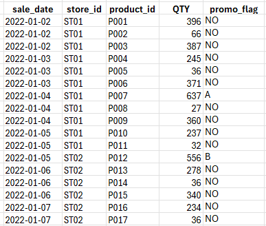
Notice what is happening. On 4th Jan, sales hit 637 units for P007 under Promotion A. Without any promotion, it settles between 300 and 350.
That is not noise. That is structure. It just requires the right variable to make it visible.
Two Models. Same Data. Very Different Futures.
The most direct way to understand what a promotion regressor does is to look at the two fit charts side by side and ask a simple question: which model actually sees the spikes?
Without the Regressor: The Model Goes Blind at the Peaks
The first model was built on the raw time series alone. No external variables. No promotional calendar. Just dates and net sales quantities fed into a forecasting pipeline.
Here is what the fit looks like:
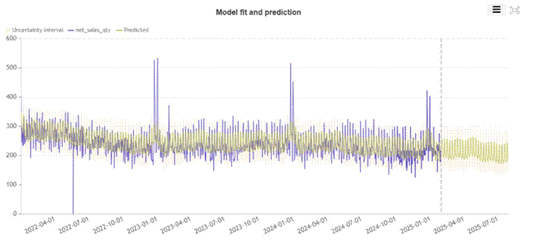
Figure 1: Model fit and prediction WITHOUT promotion regressor. The predicted line (olive/yellow) tracks the average but completely misses the promotional spikes in late 2022, early 2023, and early 2024.
Look at the three major spikes in the actual data (blue line): late December 2022, early January 2023, and late December 2023 into January 2024. The predicted line (olive) drifts through all three as if they are not there. It does not spike. It does not even react. The model has absorbed those events into its seasonal average and moved on.
The trend decomposition tells the same story from a different angle.
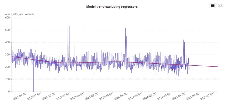
Figure 2: Underlying trend excluding regressors. A slow, steady downward drift from roughly 270 units to 200 units by mid-2025. The model has no mechanism to distinguish a promoted day from a regular one.
The underlying model sees a product in gradual decline. That may even be true on non-promoted days. But because the model cannot tell a promoted day from a normal one, its forecast for any future date is the same answer: somewhere around 170 units, trending slowly lower.
This is the forecasting equivalent of a weather model that predicts average seasonal temperature, ignoring whether a storm front is approaching.
With the Regressor: The Model Finally Sees What Is Happening
The second model added one column: promo_flag. That is all. One categorical variable encoding whether a day carries Promotion A, Promotion B, or no promotion.
Here is the same period, with the regressor included:
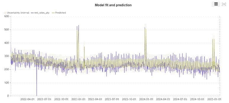
Figure 3: Model fit and prediction WITH promotion regressor. The predicted line now spikes sharply at exactly the dates where promotions occurred, closely tracking the actual peaks.
The difference is immediate. The three major promotional events that the previous model smoothed over are now captured. The predicted line rises sharply at the right moments, falls back to baseline when the promotion ends, and tracks the actual sales curve far more faithfully throughout the entire training period.
This is not overfitting. The model has not memorized individual observations. It has learned a generalizable relationship: when this flag appears, demand responds in this way. That relationship can then be applied to future dates.
The Zoom: Catching the Spike to Within 3 Units
Zooming into the December 2022 to February 2023 window makes the precision concrete.
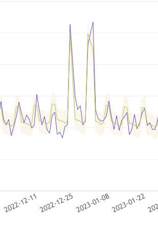
Figure 4: Zoomed view of December 2022. The model predicted 497.24 units on 2022-12-31 for SKU #ST01_#0123. The actual value was 464. Without the regressor, the model predicted roughly 240 for that same date.
A predicted value of 497 versus an actual of 464. That is an error of about 7% on a day when the no-regressor model was off by more than 100%. The model did not just notice that something happened around Christmas. It predicted almost exactly how much it would sell.
That kind of precision changes what operations can do with a forecast. Stock decisions made at 7% error versus 50% error are qualitatively different decisions.
The Numbers: Modest on Paper, Transformational in Practice
The accuracy metrics tell part of the story:
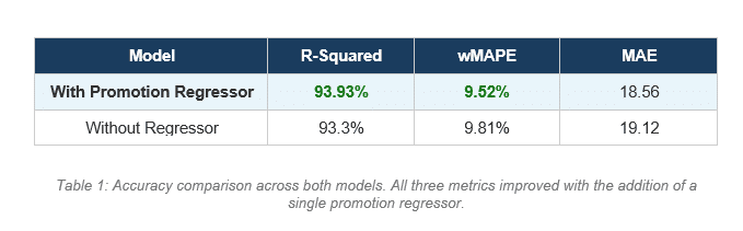
R-Squared improved from 93.3% to 93.93%. wMAPE dropped from 9.81% to 9.52%. MAE fell from 19.12 to 18.56 units per day.
The improvement looks small in percentage terms. That framing is misleading for two reasons.
First, these are aggregate metrics across the entire training period, the majority of which is non-promoted baseline days. The improvement on promoted days specifically is far larger than the aggregate suggests.
Second, and more importantly, the metric improvement is the wrong thing to focus on. The real difference is not accuracy on historical data. It is the ability to answer a question the previous model could not answer at all: what will demand be if we run this specific promotion on these specific dates?
The Forecast Became a Planning Tool
This is where the conversation changes.
Without the regressor, you ask the model: what will demand be next week? It returns a number based on trend and seasonality. That number is useful for baseline inventory planning. It is not operational.
With the regressor, you ask something different: what will demand be next week if we run Promotion A on Thursday and Promotion B on Friday?
The model can now answer that. Here is the actual API request and here is what comes back:
{
  "date": "2026-03-19",  "predicted": 388.18,  "lower": 354.09,  "upper": 420.79
  "date": "2026-03-20",  "predicted": 334.66,  "lower": 299.42,  "upper": 366.95
}
Now compare that against the baseline forecast from the model without any promotional input:
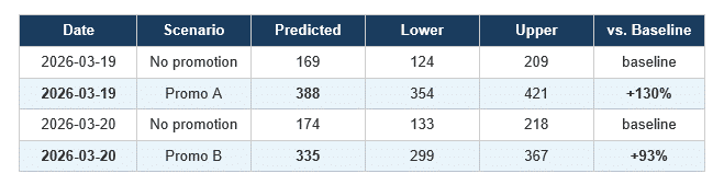
Table 2: Predicted demand with and without promotion input for the same SKU on the same dates.
The numbers are stark. On March 19th, a Promotion A day takes predicted demand from 169 units to 388 units. That is more than double. On March 20th, Promotion B lifts demand from 174 to 335, an increase of 93%.
A business planning stock without this information would order for 170 units. The actual promotional demand will be somewhere between 354 and 421. The result is either a stockout and lost revenue, or an emergency reorder at expedited freight cost.
The model with the regressor does not just produce a better number. It enables a fundamentally different planning conversation.
Promo A outperforms Promo B on this SKU. The model predicts 388 units under Promotion A versus 335 under Promotion B. If the promotional calendar is flexible, the model is telling you which promotion to run on which day. That is not forecasting. That is planning with predicted outcomes.
You can now ask which promotion type drives higher lift for this specific SKU in this specific store. You can ask whether running Promotion A on a Saturday outperforms Promotion B on a Sunday. You can simulate the full promotional calendar two weeks out and plan warehouse operations, delivery routes, and staffing accordingly.
This is the version of forecasting that connects to operational decisions. The model does not just tell you what will probably happen. It tells you what will probably happen if you do this, specifically.
The Regressor Trap: More Is Not Always Better
There is a temptation that appears in almost every forecasting project I have seen. Once the team realizes that adding a regressor improved the model, the instinct is to add more. Temperature. Competitor pricing. School holidays. Foot traffic. Exchange rates. Sentiment scores. Economic indicators.
Each one sounds reasonable. Each one might genuinely correlate with sales. The model will often accept all of them and return slightly better in-sample fit metrics.
But there is a constraint that gets forgotten in the excitement.
Every regressor you include in training must be supplied at prediction time. If you cannot provide the value for future dates with confidence, the regressor does not belong in the model.
When you train the model on promotion flags, you can query it with future promotion flags because your commercial team has a promotional calendar. They know what is planned weeks or months in advance. They can supply that value for every future date you want to forecast.
But when you train on daily temperature, you need future temperature values to generate a forecast. That means you need a weather forecast API integrated into your pipeline. Which means additional infrastructure, latency, potential data gaps, and a second source of forecast error.
When you train on competitor pricing, you need real-time competitor pricing at prediction time. Do you have that? Is it scraped daily? Is it reliable? What happens when it is unavailable?
The question to ask before adding any regressor is not “does this variable correlate with sales?” It is “can I reliably supply this variable for every future date I want to forecast?”
If the answer is no, the regressor creates a system that cannot be run in production, or one that silently fails by substituting missing values with zeros or historical means while producing forecasts that look confident but are wrong.
The promotional calendar wins not just because it correlates with demand. It wins because your business already owns the calendar, already plans it in advance, and already has someone accountable for its contents. The regressor costs almost nothing to supply. That is what makes it production-ready.
What the Model Already Understood
To be complete about what the model captures, the seasonality decomposition is worth examining even in the no-regressor version.
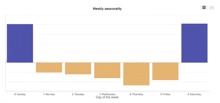
Figure 5: Weekly seasonality. Sunday and Saturday show strongly positive effects. Monday through Friday show suppressed demand, with Thursday the weakest performing weekday.
Sunday and Saturday carry significant positive multipliers. The midweek dip is real and consistent. For a parts distributor serving retail customers and weekend mechanics, this makes complete sense. The model captured this without any additional input.
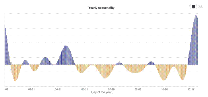
Figure 6: Yearly seasonality. Demand peaks in January and around April, with a sharp December spike. Suppressed periods in mid-summer and autumn.
The yearly seasonality catches the broad strokes. A December peak. An April uplift. Suppressed demand through summer. These are real signals.
But the model without regressors is guessing at December sales based on historical seasonal shape alone. It has no way of knowing whether this December carries a Promotion A campaign or not. Adding the regressor means it no longer has to guess. You tell it. It responds.
Diagnosis Before Prescription
Twenty years of working with data has taught me one consistent lesson. The gap between insight and action is almost never a math problem. It is a labeling problem.
The spikes in your demand data are not noise. They are events that have not been named in your dataset yet. Once you name them, the model can learn from them. Once it learns from them, it can answer questions about future planned events rather than simply extrapolating from past averages.
The promotion regressor in this case added fewer than 30 characters of information per row. Its contribution to aggregate accuracy metrics was modest. Its contribution to model utility was the difference between a passive report and an active planning engine.
A forecast that cannot be interrogated is a report. A forecast that responds to business inputs is a decision engine.
The difference is usually one column in your dataset. The harder discipline is knowing when to stop adding columns, and being honest with yourself about which ones you can actually supply when it matters.
There is an obvious question hiding in this analysis. If promotion lifts demand by 130%, why not run promotions every day?
The answer is margin. A promotion almost always means a price reduction. Selling 388 units at a discounted price may generate less gross profit than selling 169 units at full price, depending on how deep the discount goes and what the contribution margin looks like on this specific SKU. You can win on volume and lose on profit simultaneously. It happens more often than most commercial teams want to admit.
This is where demand forecasting ends and causal analysis begins. The forecast tells you what will happen to volume if you promote. It does not tell you whether that volume lift is worth the margin sacrifice, the extra inventory you had to order, the logistics cost of fulfilling a higher-demand day, or the cannibalization of full-price sales on adjacent days. Answering those questions requires estimating the net profit impact of the promotion itself, isolated from everything else happening in the business at the same time. That is a different model, built on different logic. But it starts with exactly the kind of clean, regressor-aware forecast we built here. You cannot measure the value of a decision without first being able to predict its consequences accurately.
#DemandForecasting #SupplyChain #DecisionIntelligence #RetailAnalytics #MachineLearning