| 39% → 8% Forecast error (MAPE) | 50,000+ SKUs modeled | $4.5M Annual capital impact |
CLIENT CONTEXT
The Challenge at a Glance
| Industry | Automotive Parts Distribution |
| Profile | Multi-national distributor across Central American markets, managing 50,000+ active spare parts SKUs. |
| Planning Team | 15 demand planners on ERP-native forecasting, supplemented by manual overrides and a standalone planning tool. |
| Forecast Error | 39% MAPE across the automotive portfolio · 41% across all business units. |
| Core Problem | One forecasting method across 50,000 SKUs with radically different demand behaviors — from high-turnover consumables to parts that sell twice a year. |
| Engagement | Two-phase Decision Intelligence program: proof-of-concept followed by full portfolio operationalization. |
THE PROBLEM
One Model for 50,000 SKUs. It Doesn’t Work.
The client’s ERP forecasting logic applied the same statistical method to every SKU in its portfolio, regardless of how that SKU actually behaves. A filter that sells 800 units a month and a seal that sells twice a year were treated identically. The results were predictable: inflated error rates, planners overriding the system by instinct, and no visibility into whether those overrides were helping or making things worse.
Pain points confirmed during discovery
- 39% average MAPE across the automotive SKU portfolio, confirmed from the client’s own data warehouse — rising to 41% across all business units.
- Planners overriding system forecasts at volume, with no governance layer tracking whether those overrides improved or degraded accuracy.
- No segmentation between sparse, intermittent SKUs and regular high-turnover items. Different demand regimes require fundamentally different modeling approaches.
- Fleet size (units in operation) data was available but unused. The structural driver of parts demand was invisible to the forecasting system.
- No S&OP process in the automotive business unit. No calibration loop between the forecast and actual ordering decisions.
The core finding: this was not a data problem. It was a modeling architecture problem. Applying one method to a portfolio of 50,000 SKUs with radically different demand behaviors guarantees high error regardless of how much the model is tuned.
Forecast accuracy — before and after
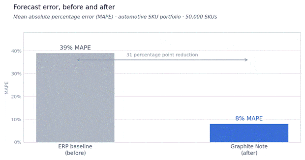
MAPE across the automotive SKU portfolio. Baseline from client’s own data warehouse vs. Graphite Note model on the same SKU set.
THE APPROACH
A Two-Phase Decision Intelligence Program
Graphite Note structured the engagement in two phases: first prove the methodology and financial impact at controlled scale, then operationalize across the full portfolio. The engagement delivers decisions, not just models.
| Objective | Timeline | Deliverables | |
| Phase 1 Core Implementation | Validate production-ready forecasting methodology using exposure-driven modeling. Prove mechanism, financial impact, and architecture. | 4–6 weeks | Validated framework · Forecast comparison · Segmentation rules · Executive presentation · Implementation blueprint |
| Phase 2 Portfolio Scale & Operationalization | Scale across the full 50,000-SKU portfolio and operationalize with automated refresh, monitoring, and ERP integration. | 8–12 weeks | Portfolio-wide forecasts · Automated regime assignment · Exposure-adjusted engine · Monitoring spec · Production-ready logic |
Portfolio segmentation by demand regime
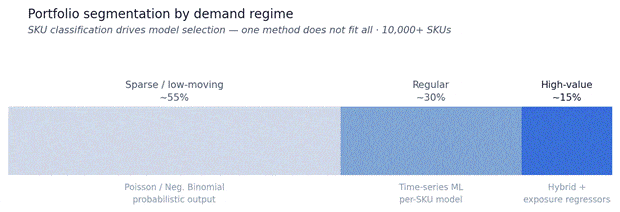
SKU classification is the foundation of the methodology. Each regime routes to a different modeling approach.
Four Principles That Drive the Methodology
One model per SKU. Every SKU receives its own trained model, capturing its individual seasonality, trend, and demand pattern. Portfolio-level averages hide the signal in every individual SKU.
Structural demand decomposition. The Fleet × Rate framework treats demand as a function of fleet size and consumption rate, converting aggregate demand into a quantity that moves predictably with the installed base.
Probabilistic treatment for sparse SKUs. Low-moving items cannot be forecast with time-series methods. Poisson and Negative Binomial distributions produce probability ranges rather than false point estimates.
White-box outputs only. Every recommendation is traceable. Planners can see exactly why the model suggests a specific order quantity and what its historical accuracy has been.
RESULTS
What the Engagement Produced
Forecast Accuracy
Initial modeling on a representative subset demonstrated forecast error in the 8% MAPE range, against the client’s confirmed 39% MAPE baseline on the same segment. This was produced in a single working session, before introducing additional regressors such as vehicle sales data or workshop order volumes.
The client evaluated whether general-purpose AI tools could handle demand forecasting at this scale. The conclusion: a large language model cannot train a dedicated model per SKU, cannot decompose individual seasonality patterns, and cannot produce the probabilistic outputs required for sparse parts.
Override Governance
A critical requirement surfaced during discovery: the client needed a governance layer for forecast overrides. With planners making manual adjustments across 50,000 SKUs, the business had no visibility into whether those adjustments were adding value or destroying it.
Override accuracy drift over time
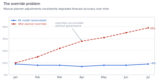
ML model accuracy remains stable while untracked planner overrides accumulate error across the planning horizon.
Financial Impact
A 50,000-SKU portfolio at an average inventory value of $3,000 per SKU represents a $150M inventory base. A 3% improvement in inventory efficiency delivers $4.5M in capital impact in Year 1 alone. Even a 1% improvement produces a return that easily justifies the engagement.
Inventory capital impact — conservative estimate
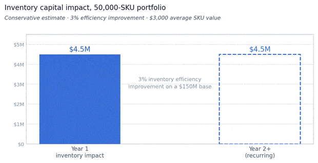
Year 1 and recurring annual impact. Based on 3% efficiency improvement on a $150M inventory base.
CLIENT VOICE
In Their Own Words
| “There is potential to improve our very bad forecast. What could differentiate you is not just the ML number, but the governance and the processes. The planning process is too manual for this portfolio size. If you can include ML in the governance part of this, I believe that is what we are looking for.” Head of Supply Chain Planning |
WHY GRAPHITE NOTE
Built for This Problem
General-purpose AI tools have no mechanism to train one model per SKU, learn individual demand seasonality, or output the probabilistic ranges required for sparse and intermittent parts. Graphite Note is purpose-built for exactly this problem.
| Per-SKU ML models | One trained model per SKU — individual seasonality and trend, not portfolio averages. |
| Automated regime routing | The platform classifies each SKU and routes it to the appropriate modeling method automatically. |
| Exposure-driven forecasting | Fleet size and usage rates incorporated as structural demand drivers, not optional add-ons. |
| White-box outputs | Planners see exactly what the model learned, its accuracy history, and why it recommends each action. |
| ISO 27001 & ISO 42001 | Certified for data security and AI governance. Enterprise-ready from day one. |
| API-first deployment | AWS-hosted, API-accessible per-SKU predictions. Refreshable weekly or daily. ERP-ready outputs. |